Fraud Detection with NebulaGraph GraphDatabase in action

Wey Gu included in category Nebula Graph

2022-08-01 2023-02-09 8100 words 39 minutes

This is a review of Fraud Detection methods based on graph algorithms, graph databases, machine learning, and graph neural networks on NebulaGraph, and in addition to an introduction to the basic methodological ideas, I've also got a Playground you can run. it's worth mentioning that this is the first time I've introduced you to the Nebula-DGL project 😁.

Contents

This is a review of Fraud Detection methods based on graph algorithms, graph databases, machine learning, and graph neural networks on NebulaGraph, and in addition to an introduction to the basic methodological ideas, I’ve also got a Playground you can run. it’s worth mentioning that this is the first time I’ve introduced you to the Nebula-DGL project 😁.

1 Fraud detection methods based on graph database

1.1 Graph Modeling

We started the modeling with the existing historical data, annotated information oriented to the relationship of the property graph. The data source could be the transaction event records, user data, and risk control annotations in the banking, e-commerce, or insurance industries in multiple table structures.

The modeling process is to abstract the entities we care about, the relationships between them, and the meaningful properties attached to both entities and relationships.

In general, persons, corporate entities, phone numbers, addresses, devices (e.g., terminal devices, network addresses, WiFi SSIDs to which terminal devices are connected, etc.), and orders are entities we started with to consider, and other information such as is_risky label, and information about persons and corporate entities (occupation, income, education, etc.) are modeled as properties of entities.

The model looks like this and the corresponding dataset could be generated with fraud-detection-datagen, with which you could generate dataset in any expected scale and community sturcture.

https://github.com/wey-gu/fraud-detection-datagen/raw/main/images/fraud_detection_graph_model.svg

1.2 Fraud detection with Graph Query

With a graph that encompasses persons, companies, historical loan application records, phone calls, and online applications for web-based devices, we can uncover some interesting information with certain graph queries directly.

In fact, many frauds are clusterred in nature. For example, a fraud ring may be a small group of people (e.g., 3 to 5 people) who collect ID information on a larger scale (e.g., 30) in an organized manner, initiate a large number of loans from multiple financial institutions at the same time, and then choose to discard the batch of IDs that have left a record of default after they have been disbursed, and then further choose the next batch of ID information as they have done.

Due to the group of frauds keeps utilizing new identity information, it’s hard to detect with historical records based blacklist mechanism. However, with the help of the patterns being queried in graph, such case could be resovled in real-time.

These patterns can be categorised into two types:

One is that which can be directly described by the risk control expert in terms of some pattern, e.g., a direct or indirect association with an entity that has been marked as high risk (new order applicants use the same network devices as past high risk records), and this pattern corresponds to the graph, which gives results in real time through a graph query.
Another type of association is implicitly behind the correlation of the data, which needs to be mined by graph algorithms for some risk hints, e.g., although a given entity has no matching association with a limited number of labeled high-risk entities, the aggregation it forms in the graph may suggest that this may be one of the applications of an ongoing gang loan fraud that has not yet succeeded, which can be derived by periodically batching in the historical data This situation can be derived by periodically performing community discovery algorithms in bulk in historical data, and using centrality algorithms in highly aggregated communities to give core entities that are prompted to risk experts for subsequent evaluation and risk labeling.

1.2.1 Fraud detection based on expert graph pattern matching

Before we get started, let’s prepare for a NebulaGraph playground with the above graph dataset being loaded:

Nebula Graph Playground setup, based on https://github.com/wey-gu/nebula-up/

1

curl -fsSL nebula-up.siwei.io/install.sh | bash

Load graph dataset

 1
 2
 3
 4
 5
 6
 7
 8
 9
10
11
12


# clone dataset genarator repo
git clone https://github.com/wey-gu/fraud-detection-datagen.git
cp -r data_sample_numerical_vertex_id data
# remove table head
sed -i '1d' data/*.csv
# load dataset to nebulagraph
docker run --rm -ti \
    --network=nebula-net \
    -v ${PWD}:/root/ \
    -v ${PWD}/data/:/data \
    vesoft/nebula-importer:v3.1.0 \
    --config /root/nebula_graph_importer.yaml

With such a mapping, risk control experts can explore the relationships between entities on-demand in a visual exploration tool that maps the corresponding risk patterns:

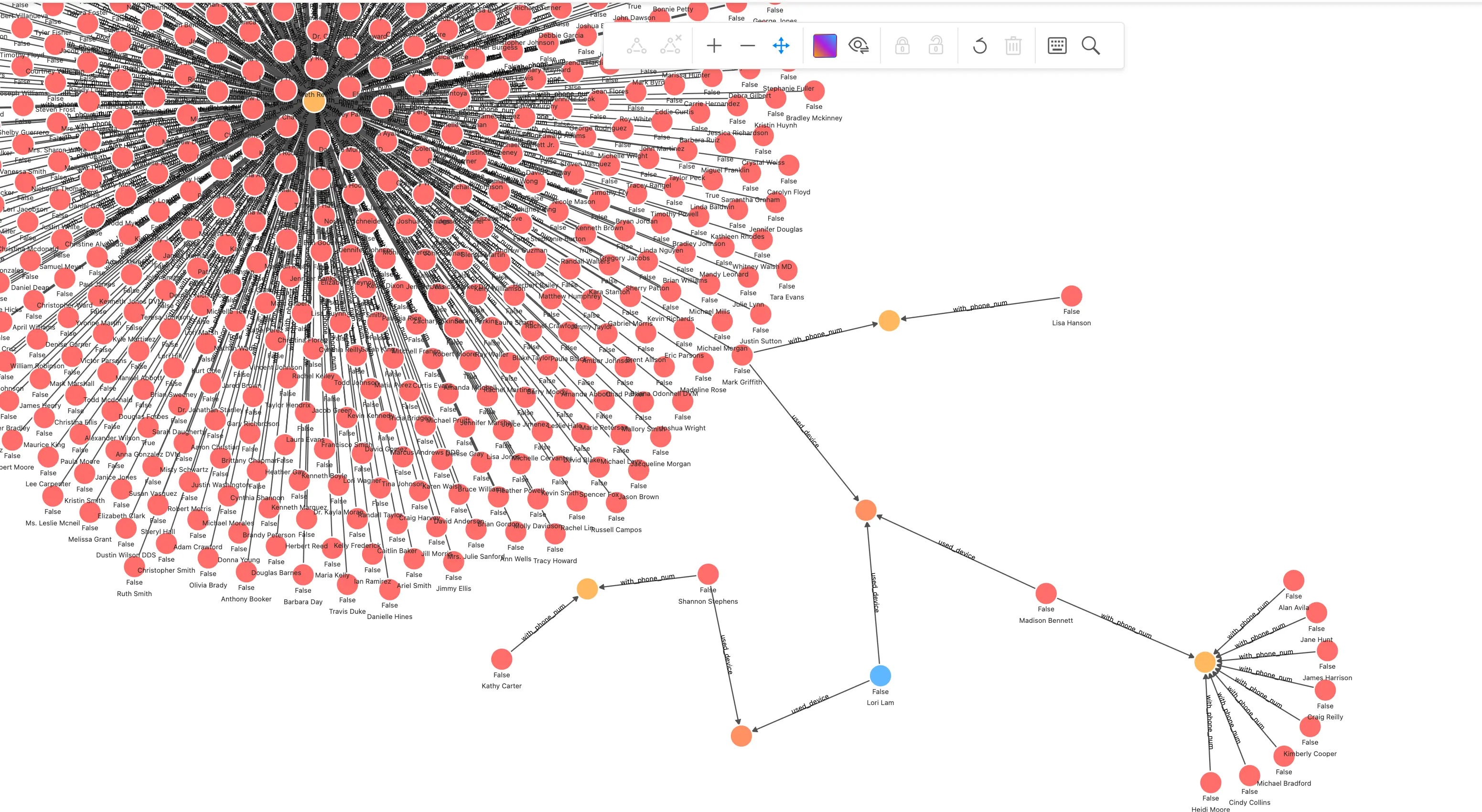
/fraud-detection-with-nebulagraph/viz_graph_query.webp

In this screenshot of rendered query, we can clearly see a risk pattern for a group-controlled device that can be given to a graph database developer and abstracted into NebulaGraph database statements that can be queried by anyone or certain application in real-time fashion:

1
2
3
4


## Query started from a person for given transaction
MATCH (n) WHERE id(n) == "200000010265"
OPTIONAL MATCH p_shared_d=(n)-[:`used_device`]->(d)<-[:`used_device`]-(:`applicant`)-[:`with_phone_num`]->(pn:`phone_num`)<-[e:`with_phone_num`]-(:`applicant`)
RETURN p_shared_d

Then we could create an API based on queries like the following, which returns count(e) as a metrics.

1
2
3
4


## group controlled device metric
MATCH (n) WHERE id(n) == "200000010265"
OPTIONAL MATCH p_shared_d=(n)-[:`used_device`]->(d)<-[:`used_device`]-(:`applicant`)-[:`with_phone_num`]->(pn:`phone_num`)<-[e:`with_phone_num`]-(:`applicant`)
RETURN count(e)

In this way, we can build an online risk control system that uses limited labeled data and expert resources to more efficiently control the risk of gang fraud.

Another example of leveraging labeled high-risk vertices could be like querying the count of ones whose is_risky flag is True:

1

MATCH p_=(p:`applicant`)-[*1..2]-(p2:`applicant`) WHERE id(p)=="200000014810" AND p2.`applicant`.is_risky == "True" RETURN p_ LIMIT 100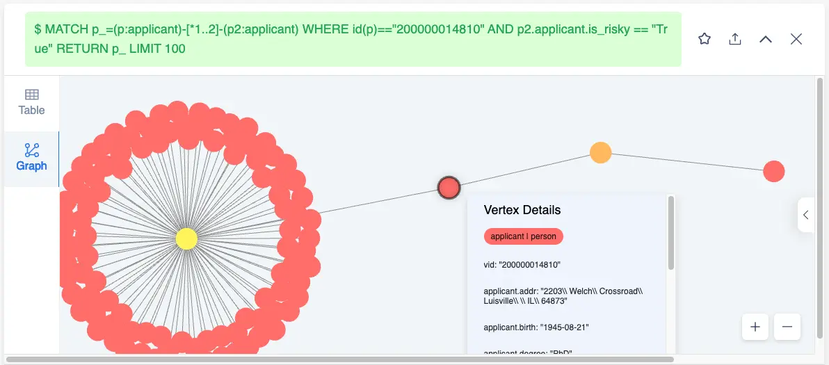

/fraud-detection-with-nebulagraph/is_risky_label.webp

And the metric would be like:

1

MATCH (p:`applicant`)-[*1..2]-(p2:`applicant`) WHERE id(p)=="200000014810" AND p2.`applicant`.is_risky == "True" RETURN count(p2)

However, in real world, most of our labeled data is still too expensive to obtain, so is there any way to more effectively use the limited risk labeling and graph structure to predict the risk?

The answer is yes.

1.3 Expand labels in Graph

In the paper: Learning from Labeled and Unlabeled Data with Label Propagation (CMU-CALD-02-107) by Xiaojin Z. and Zoubin G., the Label Propagation algorithm is used to propagate limited labeled information on the graph to more entities through the edges.

In this way, we can easily “propagate” more labeled information with a limited number of high-risk annotations in the graphs we build. These extended labeles can, on the one hand, give more results in real-time graph queries and, on the other hand, serve as important input for risk control experts to help advance anti-fraud investigation actions.

In general, we can scan the graph data offline periodically, expand and update the labels by the graph algorithm, and then write the valid updated labels back to the graph.

Note that there is a similar method, SIGNDiffusion, for those who are interested.

1.3.1 Try expanding labels in graph

Here is an example that works.

In this example, I use the public Yelp dataset. This data will not only be used in this example, but also in the later cases in the GNN method, so you can be patient and import the data into NebulaGraph.

Load dataset into NebulaGraph

More details in: https://github.com/wey-gu/nebulagraph-yelp-frauddetection

 1
 2
 3
 4
 5
 6
 7
 8
 9
10
11
12
13


git clone https://github.com/wey-gu/nebulagraph-yelp-frauddetection
cd nebulagraph-yelp-frauddetection
python3 -m pip install -r requirements.txt
# download and process dataset
python3 data_download.py

# load it into NebulaGraph
docker run --rm -ti \
    --network=nebula-net \
    -v ${PWD}/yelp_nebulagraph_importer.yaml:/root/importer.yaml \
    -v ${PWD}/data:/root \
    vesoft/nebula-importer:v3.1.0 \
    --config /root/importer.yaml

After it’s done, we could see the data stats:

1

~/.nebula-up/console.sh -e "USE yelp; SHOW STATS"

It should look like:

 1
 2
 3
 4
 5
 6
 7
 8
 9
10
11
12


(root@nebula) [(none)]> USE yelp; SHOW STATS
+---------+---------------------------------------+---------+
| Type    | Name                                  | Count   |
+---------+---------------------------------------+---------+
| "Tag"   | "review"                              | 45954   |
| "Edge"  | "shares_restaurant_in_one_month_with" | 1147232 |
| "Edge"  | "shares_restaurant_rating_with"       | 6805486 |
| "Edge"  | "shares_user_with"                    | 98630   |
| "Space" | "vertices"                            | 45954   |
| "Space" | "edges"                               | 8051348 |
+---------+---------------------------------------+---------+
Got 6 rows (time spent 1911/4488 us)

Currently, the general LPA tag propagation algorithm is used for community detection and few implementations are used for tag expansion (only SK-Learn has this implementation), here, we refer to the implementation given by [Thibaud M](https://datascience.stackexchange.com/users/77683/ thibaud-m) for the implementation given.

The orginal talks could be referred: https://datascience.stackexchange.com/a/55720/138720

To make this algorithm run faster, a subgraph is taken from the NebulaGraph and an expansion of the labeling is done on this small subgraph:

First, we start a Playground for Jupyter.

More details in: https://github.com/wey-gu/nebula-dgl.

1
2
3
4
5
6


git clone https://github.com/wey-gu/nebula-dgl.git
cd nebula-dgl
# run the Jupyter Notebook
docker run -it --name dgl -p 8888:8888 --network nebula-net \
    -v "$PWD":/home/jovyan/work jupyter/datascience-notebook \
    start-notebook.sh --NotebookApp.token='nebulagraph'

visit http://localhost:8888/lab/tree/work?token=nebulagraph

Install depednecies(they will be used in GNN examples, too)

1
2


!python3 -m pip install git+https://github.com/vesoft-inc/nebula-python.git@8c328c534413b04ccecfd42e64ce6491e09c6ca8
!python3 -m pip install .

Then, let’s sample a subgraph, starting from the vertex with ID 2048, to get all vertecies in two steps:

 1
 2
 3
 4
 5
 6
 7
 8
 9
10
11
12
13
14
15
16
17
18
19
20
21
22
23
24
25
26
27
28
29
30
31
32
33
34
35
36
37
38
39
40
41
42
43
44
45
46
47
48
49
50
51
52
53
54
55
56
57
58
59
60
61
62
63
64
65
66
67
68


import torch
import json
from torch import tensor
from dgl import DGLHeteroGraph, heterograph

from nebula3.gclient.net import ConnectionPool
from nebula3.Config import Config

config = Config()
config.max_connection_pool_size = 2
connection_pool = ConnectionPool()
connection_pool.init([('graphd', 9669)], config)

vertex_id = 2048
client = connection_pool.get_session('root', 'nebula')
r = client.execute_json(
    "USE yelp;"
    f"GET SUBGRAPH WITH PROP 2 STEPS FROM {vertex_id} YIELD VERTICES AS nodes, EDGES AS relationships;")

r = json.loads(r)
data = r.get('results', [{}])[0].get('data')
columns = r.get('results', [{}])[0].get('columns')

# create node and nodedata
node_id_map = {} # key: vertex id in NebulaGraph, value: node id in dgl_graph
node_idx = 0
features = [[] for _ in range(32)] + [[]]
for i in range(len(data)):
    for index, node in enumerate(data[i]['meta'][0]):
        nodeid = data[i]['meta'][0][index]['id']
        if nodeid not in node_id_map:
            node_id_map[nodeid] = node_idx
            node_idx += 1
            for f in range(32):
                features[f].append(data[i]['row'][0][index][f"review.f{f}"])
            features[32].append(data[i]['row'][0][index]['review.is_fraud'])

rur_start, rur_end, rsr_start, rsr_end, rtr_start, rtr_end = [], [], [], [], [], []
for i in range(len(data)):
    for edge in data[i]['meta'][1]:
        edge = edge['id']
        if edge['name'] == 'shares_user_with':
            rur_start.append(node_id_map[edge['src']])
            rur_end.append(node_id_map[edge['dst']])
        elif edge['name'] == 'shares_restaurant_rating_with':
            rsr_start.append(node_id_map[edge['src']])
            rsr_end.append(node_id_map[edge['dst']])
        elif edge['name'] == 'shares_restaurant_in_one_month_with':
            rtr_start.append(node_id_map[edge['src']])
            rtr_end.append(node_id_map[edge['dst']])

data_dict = {}
if rur_start:
    data_dict[('review', 'shares_user_with', 'review')] = tensor(rur_start), tensor(rur_end)
if rsr_start:
    data_dict[('review', 'shares_restaurant_rating_with', 'review')] = tensor(rsr_start), tensor(rsr_end)
if rtr_start:
    data_dict[('review', 'shares_restaurant_in_one_month_with', 'review')] = tensor(rtr_start), tensor(rtr_end)
# construct a dgl_graph, ref: https://docs.dgl.ai/en/0.9.x/generated/dgl.heterograph.html

dgl_graph: DGLHeteroGraph = heterograph(data_dict)

# load node features to dgl_graph
dgl_graph.ndata['label'] = tensor(features[32])

# heterogeneous graph to heterogeneous graph, keep ndata and edata
import dgl
hg = dgl.to_homogeneous(dgl_graph, ndata=['label'])

Then, let’s apply the Label Spreading algorithm mentioned above to this subgraph:

  1
  2
  3
  4
  5
  6
  7
  8
  9
 10
 11
 12
 13
 14
 15
 16
 17
 18
 19
 20
 21
 22
 23
 24
 25
 26
 27
 28
 29
 30
 31
 32
 33
 34
 35
 36
 37
 38
 39
 40
 41
 42
 43
 44
 45
 46
 47
 48
 49
 50
 51
 52
 53
 54
 55
 56
 57
 58
 59
 60
 61
 62
 63
 64
 65
 66
 67
 68
 69
 70
 71
 72
 73
 74
 75
 76
 77
 78
 79
 80
 81
 82
 83
 84
 85
 86
 87
 88
 89
 90
 91
 92
 93
 94
 95
 96
 97
 98
 99
100
101
102
103
104
105
106
107
108
109
110
111
112
113
114
115
116
117
118
119
120
121
122
123
124
125
126
127
128
129
130
131
132
133
134
135
136
137
138
139
140
141
142
143
144
145
146
147
148
149


from abc import abstractmethod
import torch

class BaseLabelPropagation:
    """Base class for label propagation models.
    
    Parameters
    ----------
    adj_matrix: torch.FloatTensor
        Adjacency matrix of the graph.
    """
    def __init__(self, adj_matrix):
        self.norm_adj_matrix = self._normalize(adj_matrix)
        self.n_nodes = adj_matrix.size(0)
        self.one_hot_labels = None 
        self.n_classes = None
        self.labeled_mask = None
        self.predictions = None

    @staticmethod
    @abstractmethod
    def _normalize(adj_matrix):
        raise NotImplementedError("_normalize must be implemented")

    @abstractmethod
    def _propagate(self):
        raise NotImplementedError("_propagate must be implemented")

    def _one_hot_encode(self, labels):
        # Get the number of classes
        classes = torch.unique(labels)
        classes = classes[classes != -1]
        self.n_classes = classes.size(0)

        # One-hot encode labeled data instances and zero rows corresponding to unlabeled instances
        unlabeled_mask = (labels == -1)
        labels = labels.clone()  # defensive copying
        labels[unlabeled_mask] = 0
        self.one_hot_labels = torch.zeros((self.n_nodes, self.n_classes), dtype=torch.float)
        self.one_hot_labels = self.one_hot_labels.scatter(1, labels.unsqueeze(1), 1)
        self.one_hot_labels[unlabeled_mask, 0] = 0

        self.labeled_mask = ~unlabeled_mask

    def fit(self, labels, max_iter, tol):
        """Fits a semi-supervised learning label propagation model.
        
        labels: torch.LongTensor
            Tensor of size n_nodes indicating the class number of each node.
            Unlabeled nodes are denoted with -1.
        max_iter: int
            Maximum number of iterations allowed.
        tol: float
            Convergence tolerance: threshold to consider the system at steady state.
        """
        self._one_hot_encode(labels)

        self.predictions = self.one_hot_labels.clone()
        prev_predictions = torch.zeros((self.n_nodes, self.n_classes), dtype=torch.float)

        for i in range(max_iter):
            # Stop iterations if the system is considered at a steady state
            variation = torch.abs(self.predictions - prev_predictions).sum().item()
            
            if variation < tol:
                print(f"The method stopped after {i} iterations, variation={variation:.4f}.")
                break

            prev_predictions = self.predictions
            self._propagate()

    def predict(self):
        return self.predictions

    def predict_classes(self):
        return self.predictions.max(dim=1).indices

class LabelPropagation(BaseLabelPropagation):
    def __init__(self, adj_matrix):
        super().__init__(adj_matrix)

    @staticmethod
    def _normalize(adj_matrix):
        """Computes D^-1 * W"""
        degs = adj_matrix.sum(dim=1)
        degs[degs == 0] = 1  # avoid division by 0 error
        return adj_matrix / degs[:, None]

    def _propagate(self):
        self.predictions = torch.matmul(self.norm_adj_matrix, self.predictions)

        # Put back already known labels
        self.predictions[self.labeled_mask] = self.one_hot_labels[self.labeled_mask]

    def fit(self, labels, max_iter=1000, tol=1e-3):
        super().fit(labels, max_iter, tol)

class LabelSpreading(BaseLabelPropagation):
    def __init__(self, adj_matrix):
        super().__init__(adj_matrix)
        self.alpha = None

    @staticmethod
    def _normalize(adj_matrix):
        """Computes D^-1/2 * W * D^-1/2"""
        degs = adj_matrix.sum(dim=1)
        norm = torch.pow(degs, -0.5)
        norm[torch.isinf(norm)] = 1
        return adj_matrix * norm[:, None] * norm[None, :]

    def _propagate(self):
        self.predictions = (
            self.alpha * torch.matmul(self.norm_adj_matrix, self.predictions)
            + (1 - self.alpha) * self.one_hot_labels
        )
    
    def fit(self, labels, max_iter=1000, tol=1e-3, alpha=0.5):
        """
        Parameters
        ----------
        alpha: float
            Clamping factor.
        """
        self.alpha = alpha
        super().fit(labels, max_iter, tol)
        
import pandas as pd
import numpy as np
import networkx as nx
import matplotlib.pyplot as plt

nx_hg = hg.to_networkx()
adj_matrix = nx.adjacency_matrix(nx_hg).toarray()
labels = hg.ndata['label']
# Create input tensors
adj_matrix_t = torch.FloatTensor(adj_matrix)
labels_t = torch.LongTensor(labels)

# Learn with Label Propagation
label_propagation = LabelPropagation(adj_matrix_t)
print("Label Propagation: ", end="")
label_propagation.fit(labels_t)
label_propagation_output_labels = label_propagation.predict_classes()

# Learn with Label Spreading
label_spreading = LabelSpreading(adj_matrix_t)
print("Label Spreading: ", end="")
label_spreading.fit(labels_t, alpha=0.8)
label_spreading_output_labels = label_spreading.predict_classes()

Let’s render label spread in color:

 1
 2
 3
 4
 5
 6
 7
 8
 9
10
11
12
13
14
15
16
17
18
19
20
21
22
23
24
25
26
27
28


color_map = {0: "blue", 1: "green"}
input_labels_colors = [color_map[int(l)] for l in labels]
lprop_labels_colors = [color_map[int(l)] for l in label_propagation_output_labels.numpy()]
lspread_labels_colors = [color_map[int(l)] for l in label_spreading_output_labels.numpy()]

plt.figure(figsize=(14, 6))
ax1 = plt.subplot(1, 4, 1)
ax2 = plt.subplot(1, 4, 2)
ax3 = plt.subplot(1, 4, 3)

ax1.title.set_text("Raw data (2 classes)")
ax2.title.set_text("Label Propagation")
ax3.title.set_text("Label Spreading")

pos = nx.spring_layout(nx_hg)
nx.draw(nx_hg, ax=ax1, pos=pos, node_color=input_labels_colors, node_size=50)
nx.draw(nx_hg, ax=ax2, pos=pos, node_color=lprop_labels_colors, node_size=50)
nx.draw(nx_hg, ax=ax3, pos=pos, node_color=lspread_labels_colors, node_size=50)

# Legend
ax4 = plt.subplot(1, 4, 4)
ax4.axis("off")
legend_colors = ["orange", "blue", "green", "red", "cyan"]
legend_labels = ["unlabeled", "class 0", "class 1", "class 2", "class 3"]
dummy_legend = [ax4.plot([], [], ls='-', c=c)[0] for c in legend_colors]
plt.legend(dummy_legend, legend_labels)

plt.show()

It looks like this:

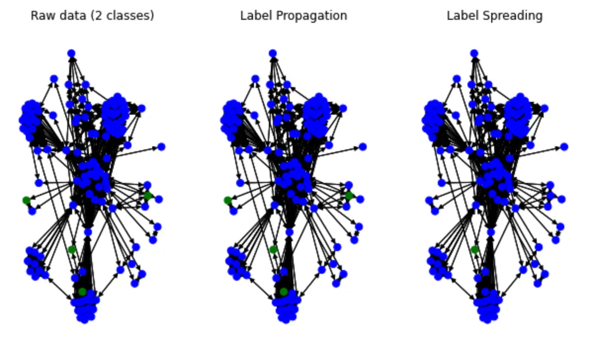
/fraud-detection-with-nebulagraph/lpa_spread_notation_matplot.webp

We could see some of the label was spread(color change).

1.4 Machine Learning with Graph Features

Before the field of risk control started to leverage the methods of the graph, there have been many approaches to predict high-risk behavior based on historical data using machine learning classification algorithms that use information in records that domain experts consider relevant (e.g., age, education, income) as features and historical label information to train risk prediction models.

So reading this, does it occur to us that on top of these methods, models trained as features might be more effective if attributes based on graph structure were also taken into account?

The answer is also yes, and there have been many papers and engineering practices revealing that such models are more effective than algorithms that do not consider graph features: these graph structure features that are tried to be effective could be PageRank values of entities, Degree values, or community ids derived from one of the community discovery algorithms.

In production, we can periodically obtain real-time full graph information from the graph, analyze it in a graph computing platform to obtain the required features, go through a predefined data pipeline, import it into a machine learning model cycle to obtain new risk cues, and write some of the results back to the graph for easy extraction and reference by other systems and experts.

1.4.1 Example of ML with Graph Features

Here, I will not demonstrate the end-to-end machine learning example, which is a common classification approach, on top of which we can get some new properties in the data by graph algorithms, which are then processed as new features. I will only demonstrate a community discovery method where we can run a Louvain on the full graph, derive the community identity of different nodes, and then process the community values as a classification into numerical features.

In this example we also use the data from https://github.com/wey-gu/fraud-detection-datagen, on top of which I used NebulaGraph-Algorithm project, a Spark application that runs many common graph algorithms on the NebulaGraph graph database.

First, let’s set up a NebulaGraph cluster with Spark and NebulaGraph Algorithm, in one-liner thanks to Nebula-UP

1

curl -fsSL nebula-up.siwei.io/all-in-one.sh | bash -s -- v3 spark

After it’s done, as I had put needed configuration files inside Nebula-UP, we could call the Louvain algorithm with:

1
2
3
4
5
6
7


cd ~/.nebula-up/nebula-up/spark && ls -l

docker exec -it sparkmaster /spark/bin/spark-submit \
    --master "local" --conf spark.rpc.askTimeout=6000s \
    --class com.vesoft.nebula.algorithm.Main \
    --driver-memory 4g /root/download/nebula-algo.jar \
    -p /root/louvain.conf

And the result will be stored in sparkmaster container, under path /output

1
2


# docker exec -it sparkmaster bash
ls -l /output

After that, we can do some pre-processing on this Louvain’s graph algorithm features and start the traditional model training.

1.5 The Graph Neural Network approach

However, the problem with these previous graph feature-based approaches is that

graph features do not fully reflect the correlations and the locality nature of the data, into our models/ methods.
graph feature engineering could be expensive and cumbersome.

In recent years, GNN-based approaches have enabled us to get better results than traditional graph feature-based machine learning by embedding graph structure and attribute information into the representation without graph feature extraction, feature engineering, and data annotation by experts and engineering methods. Interestingly, this is the period when these methods are rapidly being discovered and evolving, and graph-based deep learning is one of the hottest machine learning research directions in the previous years.

At the same time, some methods of graph deep learning can do Inductive Learning - models can inference/reason on new points and edges, so that, together with the ability to query subgraphs on the graph database online, online real-time risk prediction becomes simple and feasible.

1.5.1 Example of GNN fraud detection system

The storage of data can be in several other common media, but the graph database can maximize the benefit of model training, model updating, and online results updating. When we use the graph database as the single source of truth for the data, all online, offline, and graph-based approaches can be easily integrated to combine the advantages and results of all approaches to make a more effective composite system for fraud detection.

In this example we are divided into the same parts: Data processing, Model training, Building an online detection system.

Note, I will use Deep Graph library(DGL), NebulaGraph and the bridge between them: Nebula-DGL.

DGL: https://www.dgl.ai/

Nebula-DGL: https://github.com/wey-gu/nebula-dgl, and yes, I am the author of this project :).

1.5.1.1 Dataset

In this case, the dataset we use is Yelp-Fraud, who comes from the paper [Enhancing Graph Neural Network-based Fraud Detectors against Camouflaged Fraudsters](https:// paperswithcode.com/paper/enhancing-graph-neural-network-based-fraud).

There is one type of vertex in this diagram and three types of edges.

Top points: reviews from restaurants, hotels in Yelp with two types of attributes.
- Each review has a label labeled whether it is a false or fraudulent review
- 32 numeric attributes that have been processed
Edge: the association between the three types of reviews
- R-U-R: two reviews issued by the same user shares_user_with
- R-S-R: two reviews by the same restaurant with the same rating (rating can be 1 to 5) shares_restaurant_rating_with
- R-T-R: two ratings are from the same restaurant in the same month of submission shares_restaurant_in_one_month_with

Before we start, it’s asumed this grpah is already loaded into NebulaGraph.

To load yelp dataset into NeublaGraph, in short, you just do:

 1
 2
 3
 4
 5
 6
 7
 8
 9
10
11
12
13
14
15
16
17


# Deploy NebulaGraph
curl -fsSL nebula-up.siwei.io/install.sh | bash

# Clone the datadownloader repo
git clone https://github.com/wey-gu/nebulagraph-yelp-frauddetection && cd nebulagraph-yelp-frauddetection

# Install dep
python3 -m pip install -r requirements.txt
python3 data_download.py

# load it into NebulaGraph
docker run --rm -ti \
 --network=nebula-net \
 -v ${PWD}/yelp_nebulagraph_importer.yaml:/root/importer.yaml \
 -v ${PWD}/data:/root \
 vesoft/nebula-importer:v3.1.0 \
 --config /root/importer.yaml

More detilas in: https://github.com/wey-gu/nebulagraph-yelp-frauddetection

1.5.1.2 Data Processing

The task of this part is to engineer the topological representation of the risk-related subgraphs of the graph and the related features (attributes) in them, and serialize them into graph objects of the DGL.

DGL itself supports constructing its graph objects from CSV files in the form of point and edge lists (edgelist), or from data in the serialized sparse adjacency matrix of NetworkX and SciPy, and we can export the raw graph data or the full amount of data in the graph library to these forms. However, in the real case the data in the library is changing in real time and it is generally better to do GNN training directly on the subgraphs in NebulaGraph. Thanks to the Nebula-DGL library, this is a natural thing to do.

Note, the DGL external datamaster import documentation: https://docs.dgl.ai/guide/graph-external.html

Now let’s start this data import, before that I’ll introduce Nebula-DGL.

Nebula-DGL can construct graph objects as DGL by processing vertices, edges, and their properties in NebulaGraph into vertecies, edges, and their labels and features according to the given mapping and transformation rules (YAML format). Among them, it is worth mentioning the property-to-feature conversion.

As we know, a feature can be:

The value of a property
The value of one or more properties with certain mathematical transformations
The output of a character property as a number according to enumeration rules

Thus, they can be expressed in the Nebula-DGL API using filter for each of these cases, and let’s see how this could be done in examples:

Featre extracted directly from value of vertex/edge property

In this example, the edge type follow will be extracted, where the property degree’s value will be treated as a feature directly, and its expression in Nebula-DGL is:

 1
 2
 3
 4
 5
 6
 7
 8
 9
10
11
12


edge_types:
  - name: follow
    start_vertex_tag: player
    end_vertex_tag: player
    features:
      - name: degree
        properties:
          - name: degree
            type: int
            nullable: False
        filter:
          type: value

Feature comes from mathematical transformations of properties

In this example, we take the two properties in the serve edge and process (end_year - start_year) / 30 to become a feature called service_time.

 1
 2
 3
 4
 5
 6
 7
 8
 9
10
11
12
13
14
15
16
17


edge_types:
  - name: serve
    start_vertex_tag: player
    end_vertex_tag: team
    features:
      - name: service_time
        properties:
          - name: start_year
            type: int
            nullable: False
          - name: end_year
            type: int
            nullable: False
        # The variable was mapped by order of properties
        filter:
          type: function
          function: "lambda start_year, end_year: (end_year - start_year) / 30"

Enumerated property values into numeric features

In this example, we enumerate the name perperty in the team vertex, based on the whether they are east cost or west coast.

 1
 2
 3
 4
 5
 6
 7
 8
 9
10
11
12
13
14
15
16
17
18


vertex_tags:
  - name: team
    features:
      - name: coast
        properties:
          - name: name
            type: str
            nullable: False
        filter:
          # 0 stand for the east coast, 1 stand for the west coast
          type: enumeration
          enumeration:
            Celtics: 0
            Nets: 0
            Nuggets: 1
            Timberwolves: 1
            Thunder: 1
# ... not showing all teams here

Now we could see the trasforming API of Neubla-DGL is quite straightforward, and you could see full examples with details in https://github.com/wey-gu/nebula-dgl/tree/main/example.

With this transforming API being undsood, let’s started to process the Yelp dataset:

First, let’s define this transforming rule, where, we transform TAG: review and all three EDGE Types, with their properties values directly transforming into features:

nebulagraph_yelp_dgl_mapper.yaml

 1
 2
 3
 4
 5
 6
 7
 8
 9
10
11
12
13
14
15
16
17
18
19
20
21
22
23
24
25
26
27
28
29
30
31
32
33
34
35
36
37
38
39
40
41
42
43
44
45
46
47
48
49


---
# If vertex id is string-typed, remap_vertex_id must be true.
remap_vertex_id: True
space: yelp
# str or int
vertex_id_type: int
vertex_tags:
  - name: review
    label:
      name: is_fraud
      properties:
        - name: is_fraud
          type: int
          nullable: False
      filter:
        type: value
    features:
      - name: f0
        properties:
          - name: f0
            type: float
            nullable: False
        filter:
          type: value
      - name: f1
        properties:
          - name: f1
            type: float
            nullable: False
        filter:
          type: value
# ...
      - name: f31
        properties:
          - name: f31
            type: float
            nullable: False
        filter:
          type: value
edge_types:
  - name: shares_user_with
    start_vertex_tag: review
    end_vertex_tag: review
  - name: shares_restaurant_rating_with
    start_vertex_tag: review
    end_vertex_tag: review
  - name: shares_restaurant_in_one_month_with
    start_vertex_tag: review
    end_vertex_tag: review

Then, after nebula-dgl being installed, we could construct a DGL DGLHeteroGraph in these following lines:

 1
 2
 3
 4
 5
 6
 7
 8
 9
10
11
12
13
14
15
16
17
18
19
20
21
22


from nebula_dgl import NebulaLoader


nebula_config = {
    "graph_hosts": [
                ('graphd', 9669),
                ('graphd1', 9669),
                ('graphd2', 9669)
            ],
    "nebula_user": "root",
    "nebula_password": "nebula",
}

# load feature_mapper from yaml file
with open('nebulagraph_yelp_dgl_mapper.yaml', 'r') as f:
    feature_mapper = yaml.safe_load(f)

nebula_loader = NebulaLoader(nebula_config, feature_mapper)
g = nebula_loader.load()

g = g.to('cpu')
device = torch.device('cpu')

1.5.1.3 Model Training

Here, I use the Node Classification method of the GraphSAGE algorithm as an example, the original version of GraphSAGE is an Inductive Learning algorithm.

An Inductive Learning algorithm, which is distinguished from its opposite: Transductive Learning, means that new data can be used on top of a completely old graph to acquire a model so that the trained model can be used for online incremental data fraud detection (instead of needing to be reloaded to the full graph for training).

Model training system (left).

Input: A historical transaction graph with fraud annotation
Output: A GraphSAGE DGL model

Online inference system (right).

Model: GraphSAGE-based training based on historical transaction graphs with fraud annotations
Input: A new transaction
Output: Whether the transaction is suspected of being fraudulent

Dataset split

The process of machine learning training requires partitioning the already available data, information for training, validation and testing subsets, they can be either disjoint true subsets of the overall data or overlap each other.

In practice, sometimes our labeling of data is often inadequate, so it may make more sense to partition the data according to the proportion of labeling, the following example I segmented the dataset according to whether the vertices are labeled with fraud or not.

There are two points worth noting here.

stratify=g.ndata['is_fraud'] in train_test_split represents to keep the distribution of the values of is_fraud to split, which is in line with the idea we mentioned above.
we split the idx index, so that we can end up with three sets of indexes for training, validation and testing. At the same time, we also put the corresponding set of masks into the graph object g.

 1
 2
 3
 4
 5
 6
 7
 8
 9
10
11
12
13
14
15
16
17
18
19
20
21
22
23
24
25
26
27
28
29
30
31
32
33
34
35
36
37
38
39
40
41


# Split the graph into train, validation, and test sets

import pandas as pd
import numpy as np
from sklearn.model_selection import train_test_split

# features are g.ndata['f0'], g.ndata['f1'], g.ndata['f2'], ... g.ndata['f31']
# label is in g.ndata['is_fraud']

# concatenate all features
features = []
for i in range(32):
    features.append(g.ndata['f' + str(i)])

g.ndata['feat'] = torch.stack(features, dim=1)
g.ndata['label'] = g.ndata['is_fraud']
# numpy array as an index of range n

idx = torch.tensor(np.arange(g.number_of_nodes()), device=device, dtype=torch.int64)

# split based on value distribution of label: the property "is_fraud", which is a binary variable.
X_train_and_val_idx, X_test_idx, y_train_and_val, y_test = train_test_split(
    idx, g.ndata['is_fraud'], test_size=0.2, random_state=42, stratify=g.ndata['is_fraud'])

# split train and val
X_train_idx, X_val_idx, y_train, y_val = train_test_split(
    X_train_and_val_idx, y_train_and_val, test_size=0.2, random_state=42, stratify=y_train_and_val)

# list of index to mask
train_mask = torch.zeros(g.number_of_nodes(), dtype=torch.bool)
train_mask[X_train_idx] = True

val_mask = torch.zeros(g.number_of_nodes(), dtype=torch.bool)
val_mask[X_val_idx] = True

test_mask = torch.zeros(g.number_of_nodes(), dtype=torch.bool)
test_mask[X_test_idx] = True

g.ndata['train_mask'] = train_mask
g.ndata['val_mask'] = val_mask
g.ndata['test_mask'] = test_mask

Heterogeneous graph to Homogeneous graph

GraphSAGE is an algorithm for Homogeneous graphs with no feature on edges, while our current Yelp graph is Heterogeneous: one type of vertex(TAG) and three types of edges. So, how can we use GraphSAGE to model Yelp graphs?

Instead of finding another Inductive Learning to supports heterogeneous graphs, I actually find a way to convert homogeneous graph into a heterogeneous one. In order not to lose important edge type information in the conversion, we can make the edge type numeric.

Here I have given a one-dimensional edge feature, but of course (3-1) two-dimensional is also possible.

1
2
3


# shares_restaurant_in_one_month_with: 1, b"001"
# shares_restaurant_rating_with: 2, b"010"
# shares_user_with: 4, b"100"

Note: we could directly parse 3-type of edges mapped to [0, 1, 2] from hg.edata['_TYPE'], referring to https://docs.dgl.ai/en/0.9.x/generated/dgl.to_homogeneous.html, while I chose not to do so due to 0 cannot be appied to edge weight(it will end up 0 value in message passsing for this 0 type).

 1
 2
 3
 4
 5
 6
 7
 8
 9
10
11
12
13
14
15
16
17
18
19
20
21
22
23
24


# three types of edges
In [1]: g.etypes
Out[1]:
['shares_restaurant_in_one_month_with',
 'shares_restaurant_rating_with',
 'shares_user_with']

In [2]:
g.edges['shares_restaurant_in_one_month_with'].data['he'] = torch.ones(
    g.number_of_edges('shares_restaurant_in_one_month_with'), dtype=torch.int64)
g.edges['shares_restaurant_rating_with'].data['he'] = torch.full(
    (g.number_of_edges('shares_restaurant_rating_with'),), 2, dtype=torch.int64)
g.edges['shares_user_with'].data['he'] = torch.full(
    (g.number_of_edges('shares_user_with'),), 4, dtype=torch.int64)

In [3]: g.edata['he']
Out[3]:
{('review',
  'shares_restaurant_in_one_month_with',
  'review'): tensor([1, 1, 1,  ..., 1, 1, 1]),
 ('review',
  'shares_restaurant_rating_with',
  'review'): tensor([2, 2, 2,  ..., 2, 2, 2]),
 ('review', 'shares_user_with', 'review'): tensor([4, 4, 4,  ..., 4, 4, 4])}

ref: https://discuss.dgl.ai/t/how-to-convert-from-a-heterogeneous-graph-to-a-homogeneous-graph-with-data/2764

Then transform it to a homogeneous graph, with he as kept edata

1

hg = dgl.to_homogeneous(g, edata=['he'], ndata=['feat', 'label', 'train_mask', 'val_mask', 'test_mask'])

ref: https://docs.dgl.ai/en/latest/guide/graph-heterogeneous.html?highlight=to_homogeneous#converting-heterogeneous-graphs-to-homogeneous-graphs

The vanilla GraphSAGE implementation in dgl doesn’t consider edge feature, thus I override/changed that message passing part of code, which will be revealed later.

Ref

https://discuss.dgl.ai/t/frequently-asked-questions-faq/1681 （Question 13）

https://discuss.dgl.ai/t/using-node-and-edge-features-in-message-passing/762

Code of model training

We could refer to the dgl example of graphsage: https://github.com/dmlc/dgl/tree/master/examples/pytorch/graphsage.

As our graph comes with edge feature(due to the conversion), we could modify GraphSAGE in two ways:

a. Considering edge features, for example, if mean aggreation is used, change could be:

1
2
3
4


  graph.update_all(msg_fn, fn.mean('m', 'neigh'))
+ graph.update_all(fn.copy_e('he', 'm'), fn.mean('m', 'neigh'))
- h_neigh = graph.dstdata['neigh']
+ h_neigh = torch.cat((graph.dstdata['neigh'], graph.dstdata['neigh_e'].reshape(-1, 1)), 1)

Note that, apart from the above change, the feature dimension should be taken care, too.

b. Treate edge feature as edge weight:

1
2
3


- graph.update_all(msg_fn, fn.mean('m', 'neigh'))
+ # consdier datatype with different weight, g.edata['he'] as weight here
+ g.update_all(fn.u_mul_e('h', 'he', 'm'), fn.mean('m', 'h'))

Here, I’ll do it in b. as weight, with mean aggration:

Override the SAGEConv：

With only the Message Passing part changed.

  1
  2
  3
  4
  5
  6
  7
  8
  9
 10
 11
 12
 13
 14
 15
 16
 17
 18
 19
 20
 21
 22
 23
 24
 25
 26
 27
 28
 29
 30
 31
 32
 33
 34
 35
 36
 37
 38
 39
 40
 41
 42
 43
 44
 45
 46
 47
 48
 49
 50
 51
 52
 53
 54
 55
 56
 57
 58
 59
 60
 61
 62
 63
 64
 65
 66
 67
 68
 69
 70
 71
 72
 73
 74
 75
 76
 77
 78
 79
 80
 81
 82
 83
 84
 85
 86
 87
 88
 89
 90
 91
 92
 93
 94
 95
 96
 97
 98
 99
100
101
102
103
104
105
106
107
108
109
110
111
112
113
114


from dgl import function as fn
from dgl.utils import check_eq_shape, expand_as_pair

class SAGEConv(dglnn.SAGEConv):
    def forward(self, graph, feat, edge_weight=None):
        r"""

        Description
        -----------
        Compute GraphSAGE layer.

        Parameters
        ----------
        graph : DGLGraph
            The graph.
        feat : torch.Tensor or pair of torch.Tensor
            If a torch.Tensor is given, it represents the input feature of shape
            :math:`(N, D_{in})`
            where :math:`D_{in}` is size of input feature, :math:`N` is the number of nodes.
            If a pair of torch.Tensor is given, the pair must contain two tensors of shape
            :math:`(N_{in}, D_{in_{src}})` and :math:`(N_{out}, D_{in_{dst}})`.
        edge_weight : torch.Tensor, optional
            Optional tensor on the edge. If given, the convolution will weight
            with regard to the message.

        Returns
        -------
        torch.Tensor
            The output feature of shape :math:`(N_{dst}, D_{out})`
            where :math:`N_{dst}` is the number of destination nodes in the input graph,
            :math:`D_{out}` is the size of the output feature.
        """
        self._compatibility_check()
        with graph.local_scope():
            if isinstance(feat, tuple):
                feat_src = self.feat_drop(feat[0])
                feat_dst = self.feat_drop(feat[1])
            else:
                feat_src = feat_dst = self.feat_drop(feat)
                if graph.is_block:
                    feat_dst = feat_src[:graph.number_of_dst_nodes()]
            msg_fn = fn.copy_src('h', 'm')
            if edge_weight is not None:
                assert edge_weight.shape[0] == graph.number_of_edges()
                graph.edata['_edge_weight'] = edge_weight
                msg_fn = fn.u_mul_e('h', '_edge_weight', 'm')

            h_self = feat_dst

            # Handle the case of graphs without edges
            if graph.number_of_edges() == 0:
                graph.dstdata['neigh'] = torch.zeros(
                    feat_dst.shape[0], self._in_src_feats).to(feat_dst)

            # Determine whether to apply linear transformation before message passing A(XW)
            lin_before_mp = self._in_src_feats > self._out_feats

            # Message Passing
            if self._aggre_type == 'mean':
                graph.srcdata['h'] = self.fc_neigh(feat_src) if lin_before_mp else feat_src
                # graph.update_all(msg_fn, fn.mean('m', 'neigh'))
                #########################################################################
                # consdier datatype with different weight, g.edata['he'] as weight here
                g.update_all(fn.u_mul_e('h', 'he', 'm'), fn.mean('m', 'h'))
                #########################################################################
                h_neigh = graph.dstdata['neigh']
                if not lin_before_mp:
                    h_neigh = self.fc_neigh(h_neigh)
            elif self._aggre_type == 'gcn':
                check_eq_shape(feat)
                graph.srcdata['h'] = self.fc_neigh(feat_src) if lin_before_mp else feat_src
                if isinstance(feat, tuple):  # heterogeneous
                    graph.dstdata['h'] = self.fc_neigh(feat_dst) if lin_before_mp else feat_dst
                else:
                    if graph.is_block:
                        graph.dstdata['h'] = graph.srcdata['h'][:graph.num_dst_nodes()]
                    else:
                        graph.dstdata['h'] = graph.srcdata['h']
                graph.update_all(msg_fn, fn.sum('m', 'neigh'))
                graph.update_all(fn.copy_e('he', 'm'), fn.sum('m', 'neigh'))
                # divide in_degrees
                degs = graph.in_degrees().to(feat_dst)
                h_neigh = (graph.dstdata['neigh'] + graph.dstdata['h']) / (degs.unsqueeze(-1) + 1)
                if not lin_before_mp:
                    h_neigh = self.fc_neigh(h_neigh)
            elif self._aggre_type == 'pool':
                graph.srcdata['h'] = F.relu(self.fc_pool(feat_src))
                graph.update_all(msg_fn, fn.max('m', 'neigh'))
                graph.update_all(fn.copy_e('he', 'm'), fn.max('m', 'neigh'))
                h_neigh = self.fc_neigh(graph.dstdata['neigh'])
            elif self._aggre_type == 'lstm':
                graph.srcdata['h'] = feat_src
                graph.update_all(msg_fn, self._lstm_reducer)
                h_neigh = self.fc_neigh(graph.dstdata['neigh'])
            else:
                raise KeyError('Aggregator type {} not recognized.'.format(self._aggre_type))

            # GraphSAGE GCN does not require fc_self.
            if self._aggre_type == 'gcn':
                rst = h_neigh
            else:
                rst = self.fc_self(h_self) + h_neigh

            # bias term
            if self.bias is not None:
                rst = rst + self.bias

            # activation
            if self.activation is not None:
                rst = self.activation(rst)
            # normalization
            if self.norm is not None:
                rst = self.norm(rst)
            return rst

Define the model structure

 1
 2
 3
 4
 5
 6
 7
 8
 9
10
11
12
13
14
15
16
17
18
19
20
21
22
23
24
25
26
27
28
29
30
31
32
33
34
35
36
37
38
39
40
41
42
43
44
45
46
47


class SAGE(nn.Module):
    def __init__(self, in_size, hid_size, out_size):
        super().__init__()
        self.layers = nn.ModuleList()
        # three-layer GraphSAGE-mean
        self.layers.append(dglnn.SAGEConv(in_size, hid_size, 'mean'))
        self.layers.append(dglnn.SAGEConv(hid_size, hid_size, 'mean'))
        self.layers.append(dglnn.SAGEConv(hid_size, out_size, 'mean'))
        self.dropout = nn.Dropout(0.5)
        self.hid_size = hid_size
        self.out_size = out_size

    def forward(self, blocks, x):
        h = x
        for l, (layer, block) in enumerate(zip(self.layers, blocks)):
            h = layer(block, h)
            if l != len(self.layers) - 1:
                h = F.relu(h)
                h = self.dropout(h)
        return h

    def inference(self, g, device, batch_size):
        """Conduct layer-wise inference to get all the node embeddings."""
        feat = g.ndata['feat']
        sampler = MultiLayerFullNeighborSampler(1, prefetch_node_feats=['feat'])
        dataloader = DataLoader(
                g, torch.arange(g.num_nodes()).to(g.device), sampler, device=device,
                batch_size=batch_size, shuffle=False, drop_last=False,
                num_workers=0)
        buffer_device = torch.device('cpu')
        pin_memory = (buffer_device != device)

        for l, layer in enumerate(self.layers):
            y = torch.empty(
                g.num_nodes(), self.hid_size if l != len(self.layers) - 1 else self.out_size,
                device=buffer_device, pin_memory=pin_memory)
            feat = feat.to(device)
            for input_nodes, output_nodes, blocks in tqdm.tqdm(dataloader):
                x = feat[input_nodes]
                h = layer(blocks[0], x) # len(blocks) = 1
                if l != len(self.layers) - 1:
                    h = F.relu(h)
                    h = self.dropout(h)
                # by design, our output nodes are contiguous
                y[output_nodes[0]:output_nodes[-1]+1] = h.to(buffer_device)
            feat = y
        return y

The train, infer function:

 1
 2
 3
 4
 5
 6
 7
 8
 9
10
11
12
13
14
15
16
17
18
19
20
21
22
23
24
25
26
27
28
29
30
31
32
33
34
35
36
37
38
39
40
41
42
43
44
45
46
47
48
49
50
51
52


def evaluate(model, graph, dataloader):
    model.eval()
    ys = []
    y_hats = []
    for it, (input_nodes, output_nodes, blocks) in enumerate(dataloader):
        with torch.no_grad():
            x = blocks[0].srcdata['feat']
            ys.append(blocks[-1].dstdata['label'])
            y_hats.append(model(blocks, x))
    return MF.accuracy(torch.cat(y_hats), torch.cat(ys))

def layerwise_infer(device, graph, nid, model, batch_size):
    model.eval()
    with torch.no_grad():
        pred = model.inference(graph, device, batch_size) # pred in buffer_device
        pred = pred[nid]
        label = graph.ndata['label'][nid].to(pred.device)
        return MF.accuracy(pred, label)

def train(device, g, model, train_idx, val_idx):
    # create sampler & dataloader
    sampler = NeighborSampler([10, 10, 10],  # fanout for [layer-0, layer-1, layer-2]
                              prefetch_node_feats=['feat'],
                              prefetch_labels=['label'])
    use_uva = False
    train_dataloader = DataLoader(g, train_idx, sampler, device=device,
                                  batch_size=1024, shuffle=True,
                                  drop_last=False, num_workers=0,
                                  use_uva=use_uva)

    val_dataloader = DataLoader(g, val_idx, sampler, device=device,
                                batch_size=1024, shuffle=True,
                                drop_last=False, num_workers=0,
                                use_uva=use_uva)

    opt = torch.optim.Adam(model.parameters(), lr=1e-3, weight_decay=5e-4)
    
    for epoch in range(10):
        model.train()
        total_loss = 0
        for it, (input_nodes, output_nodes, blocks) in enumerate(train_dataloader):
            x = blocks[0].srcdata['feat']
            y = blocks[-1].dstdata['label']
            y_hat = model(blocks, x)
            loss = F.cross_entropy(y_hat, y)
            opt.zero_grad()
            loss.backward()
            opt.step()
            total_loss += loss.item()
        acc = evaluate(model, g, val_dataloader)
        print("Epoch {:05d} | Loss {:.4f} | Accuracy {:.4f} "
              .format(epoch, total_loss / (it+1), acc.item()))

Load graph from NebulaGraph into DGL

 1
 2
 3
 4
 5
 6
 7
 8
 9
10
11
12
13
14
15
16
17
18
19
20
21
22


from nebula_dgl import NebulaLoader

nebula_config = {
    "graph_hosts": [
                ('graphd', 9669),
                ('graphd1', 9669),
                ('graphd2', 9669)
            ],
    "nebula_user": "root",
    "nebula_password": "nebula",
}

with open('nebulagraph_yelp_dgl_mapper.yaml', 'r') as f:
     feature_mapper = yaml.safe_load(f)

nebula_loader = NebulaLoader(nebula_config, feature_mapper)

g = nebula_loader.load() # This will take you some time

# We use CPU as a poor guy
g = g.to('cpu')
device = torch.device('cpu')

Split dataset into training, validation and test sets, and convert it into homo graph.

 1
 2
 3
 4
 5
 6
 7
 8
 9
10
11
12
13
14
15
16
17
18
19
20
21
22
23
24
25
26
27
28
29
30
31
32
33
34
35
36
37
38
39
40
41
42
43
44
45
46
47
48
49
50
51
52
53
54
55
56
57
58


# Split the graph into train, validation and test sets

import pandas as pd
import numpy as np
from sklearn.model_selection import train_test_split

# features are g.ndata['f0'], g.ndata['f1'], g.ndata['f2'], ... g.ndata['f31']
# label is in g.ndata['is_fraud']

# concatenate all features
features = []
for i in range(32):
    features.append(g.ndata['f'+str(i)])

g.ndata['feat'] = torch.stack(features, dim=1)
g.ndata['label'] = g.ndata['is_fraud']
# numpy array as index of range n

idx = torch.tensor(np.arange(g.number_of_nodes()), device=device, dtype=torch.int64)
# features.append(idx)
# concatenate one dim with index of node
# feature_and_idx = torch.stack(features, dim=1)

# split based on value distribution of label: the property "is_fraud", which is a binary variable.
X_train_and_val_idx, X_test_idx, y_train_and_val, y_test = train_test_split(
    idx, g.ndata['is_fraud'], test_size=0.2, random_state=42, stratify=g.ndata['is_fraud'])

# split train and val
X_train_idx, X_val_idx, y_train, y_val = train_test_split(
    X_train_and_val_idx, y_train_and_val, test_size=0.2, random_state=42, stratify=y_train_and_val)

# list of index to mask
train_mask = torch.zeros(g.number_of_nodes(), dtype=torch.bool)
train_mask[X_train_idx] = True

val_mask = torch.zeros(g.number_of_nodes(), dtype=torch.bool)
val_mask[X_val_idx] = True

test_mask = torch.zeros(g.number_of_nodes(), dtype=torch.bool)
test_mask[X_test_idx] = True

g.ndata['train_mask'] = train_mask
g.ndata['val_mask'] = val_mask
g.ndata['test_mask'] = test_mask

# shares_restaurant_in_one_month_with: 1, b"001"
# shares_restaurant_rating_with: 2, b"010"
# shares_user_with: 4, b"100"
# set edata of shares_restaurant_in_one_month_with to n of 1 tensor array
g.edges['shares_restaurant_in_one_month_with'].data['he'] = torch.ones(
    g.number_of_edges('shares_restaurant_in_one_month_with'), dtype=torch.float32)
g.edges['shares_restaurant_rating_with'].data['he'] = torch.full(
    (g.number_of_edges('shares_restaurant_rating_with'),), 2, dtype=torch.float32)
g.edges['shares_user_with'].data['he'] = torch.full(
    (g.number_of_edges('shares_user_with'),), 4, dtype=torch.float32)

# heterogeneous graph to heterogeneous graph, keep ndata and edata
hg = dgl.to_homogeneous(g, edata=['he'], ndata=['feat', 'label', 'train_mask', 'val_mask', 'test_mask'])

Train and test the model

 1
 2
 3
 4
 5
 6
 7
 8
 9
10
11
12
13
14
15
16
17


# create GraphSAGE model
in_size = hg.ndata['feat'].shape[1]
out_size = 2
model = SAGE(in_size, 256, out_size).to(device)

# model training
print('Training...')
train(device, hg, model, X_train_idx, X_val_idx)

# test the model
print('Testing...')

acc = layerwise_infer(device, hg, X_test_idx, model, batch_size=4096)
print("Test Accuracy {:.4f}".format(acc.item()))

# 运行结果
# Test Accuracy 0.9996

After we have a trained model, it could be serialized as a file, and when needed, it could be loaded and used as a PyTorch model in your inference service.

1
2
3
4
5
6
7


# save model
torch.save(model.state_dict(), "fraud_d.model")

# load model
device = torch.device('cpu')
model = SAGE(32, 256, 2).to(device)
model.load_state_dict(torch.load("fraud_d.model"))

Then, let’s see how do make this model work in an online fraud detection system.

1.5.1.4 Inference API

As mentioned earlier, GraphSAGE is the simplest model to support Inductive Learning, thus our training inference process above is actually not yet the same as our test and training graphs, although the indexes of the training points are labeled, the whole graph is actually used as input.

In order to do Inductive Learning we just need to divide the training and testing into two non-intersecting subgraphs for training and final testing.

 1
 2
 3
 4
 5
 6
 7
 8
 9
10
11
12
13
14
15
16
17
18
19


# Inductive Learning, our test dataset are new nodes and new edges
hg_train = hg.subgraph(torch.cat([X_train_idx, X_val_idx]))

# model training
print('Training...')
train(device, hg_train, model, torch.arange(X_train_idx.shape[0]), torch.arange(X_train_idx.shape[0], hg_train.num_nodes()))

# test the model
print('Testing...')

hg_test = hg.subgraph(torch.cat([X_test_idx]))

sg_X_test_idx = torch.arange(hg_test.num_nodes())

acc = layerwise_infer(device, hg_test, sg_X_test_idx, model, batch_size=4096)
print("Test Accuracy {:.4f}".format(acc.item()))

# Result
# Test Accuracy 0.9990

As you can see, in our code above, the graph used for testing and the graph used for training are two completely different sets of data, which allows our online system to be data that we haven’t encountered before at all.

Thus, we can simply write the data for a new incoming transaction request into NebulaGraph and then get a small subgraph that the online system can return from that point, and use it as input to the model inference to get the labels of the subgraph!

A new trasnaction request：

Remember the flowchart of an online inference system with GNN?

 1
 2
 3
 4
 5
 6
 7
 8
 9
10
11
12
13
14
15
16
17
18
19
20
21
22
23
24
25
26
27
28


      ┌─────────────────────┐                          ┌─────────────────┐      
      │                     │                          │                 │
─────▶│ Transaction Record  ├──────2. Fraud Risk ─────▶│  Inference API  │◀────┐
      │                     │◀────Prediction with ─────┤                 │     │
      │                     │        Sub Graph         │                 │     │
      └─────────────────────┘                          └─────────────────┘     │
           │           ▲                                        │              │
           │           │                                        │              │
       0. Insert   1. Get New                              3.req: Node         │
         Record    Record Sub                            Classification        │
           │         Graph                                      │              │
           ▼           │                                        │              │
┌──────────────────────┴─────────────────┐ ┌────────────────────┘      3.resp: │
│┌──────────────────────────────────────┐│ │                          Predicted│
││   Graph of Historical Transactions   ││ │                             Risk  │
│└──────────────────────────────────────┘│ │                                   │
│                   .─.              .   │ │                                   │
│                  (   )◀───────────( )  │ │                                   │
│                   `─'              '   │ │      ┌──────────────────────┐     │
│  .       .─.       ╲             ◁     │ │      │ GNN Model Λ          │     │
│ ( )◀────(   )       ╲           ╱      │ │  ┌───┴─┐        ╱ ╲      ┌──┴──┐  │
│  '       `─'         ╲       . ╱       │ │  ├─────┤       ╱   ╲     ├─────┤  │
│  ╲       ◀            ╲     ( )        │ └─▶├─────┼─────▶▕     ─────├─────┤──┘
│   ╲  .  ╱              ◁     '         │    ├─────┤       ╲   ╱     ├─────┤   
│    ◀( )╱               .─.         .─. │    └───┬─┘        ╲ ╱      └──┬──┘   
│      '                (   )◀──────(   )│        │           V          │      
│                        `─'         `─' │        └──────────────────────┘      
└────────────────────────────────────────┘        

Now, assume a new transaction request comes to the system, and corresponding relations has been already written to the graph database, we could randomly find one review to simulate that:

1

MATCH (n:`review`) RETURN n LIMIT 1

1
2
3
4
5


+----------------------------------------------------------------------------------------------------------------------------------------------------------------------------------------------------------------------------------------------------------------------------------------------------------------------------------------------------------------------------------------------------------------------------------------------------------------------------------------------------------------------------------------------------------------------------------------------------------------------------------------------------------------------------------------------------------------------------------------------------------------------------------------------------------------------------------------+
| n                                                                                                                                                                                                                                                                                                                                                                                                                                                                                                                                                                                                                                                                                                                                                                                                                                      |
+----------------------------------------------------------------------------------------------------------------------------------------------------------------------------------------------------------------------------------------------------------------------------------------------------------------------------------------------------------------------------------------------------------------------------------------------------------------------------------------------------------------------------------------------------------------------------------------------------------------------------------------------------------------------------------------------------------------------------------------------------------------------------------------------------------------------------------------+
| (2048 :review{f0: 0.0, f1: 0.08034700155258179, f10: 0.3952670097351074, f11: 0.18671999871730804, f12: 0.2836120128631592, f13: 0.2843089997768402, f14: 0.38148200511932373, f15: 0.3816460072994232, f16: 0.9999740123748779, f17: 0.6430919766426086, f18: 0.9999740123748779, f19: 0.5051100254058838, f2: 0.12382200360298157, f20: 0.4940490126609802, f21: 0.7766339778900146, f22: 0.7705119848251343, f23: 0.9480599761009216, f24: 0.4032529890537262, f25: 0.12437800318002701, f26: 0.3184080123901367, f27: 0.5223879814147949, f28: 0.4278610050678253, f29: 0.343284010887146, f3: 0.42868199944496155, f30: 0.37313398718833923, f31: 0.328357994556427, f4: 0.9999849796295166, f5: 0.9999849796295166, f6: 0.9999849796295166, f7: 0.4850809872150421, f8: 0.454602986574173, f9: 0.8863419890403748, is_fraud: 0}) |
+----------------------------------------------------------------------------------------------------------------------------------------------------------------------------------------------------------------------------------------------------------------------------------------------------------------------------------------------------------------------------------------------------------------------------------------------------------------------------------------------------------------------------------------------------------------------------------------------------------------------------------------------------------------------------------------------------------------------------------------------------------------------------------------------------------------------------------------+

好，它是 2048 这个点。它的下一步是 1. Get New Record Subgraph 我们来获取它的子图：

OK, it’s the vertex with ID 2048, the next step in the flowchart is 1. Get New Record Subgraph , and it’s equivalent to this query:

1

GET SUBGRAPH WITH PROP FROM 2048 YIELD VERTICES AS nodes, EDGES AS relationships;

If we render the result in NebulaGraph Studio or NebulaGraph Explorer, it looks like this:

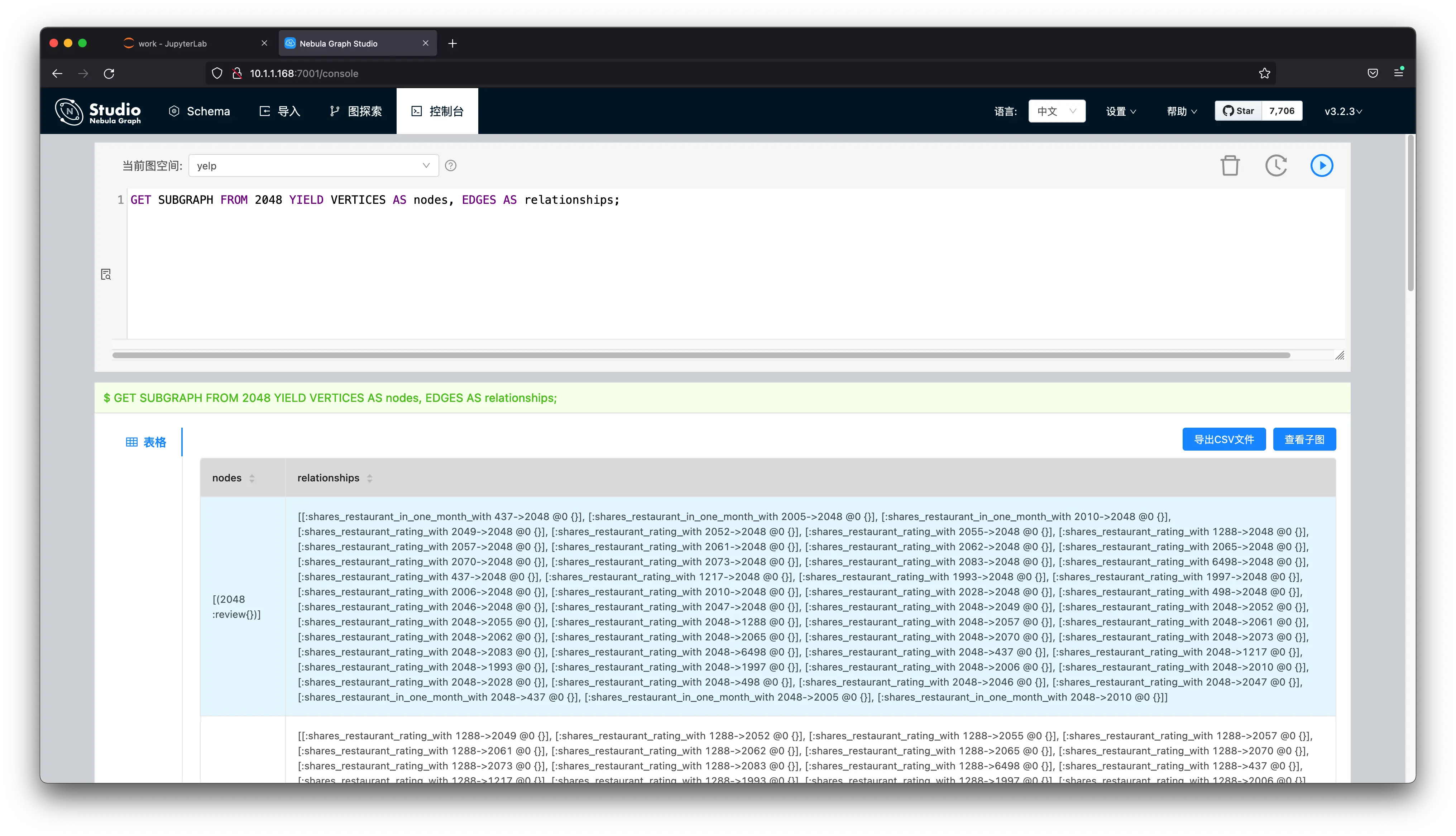
/fraud-detection-with-nebulagraph/subgraph_console_view.webp

/fraud-detection-with-nebulagraph/subgraph_viz.webp

Below is the code for the SUBGRAPH fetching, the input is vertex_id, and output is a dgl graph, which will be sent to the inference API.

 1
 2
 3
 4
 5
 6
 7
 8
 9
10
11
12
13
14
15
16
17
18
19
20
21
22


# get SUBGRAPH of one node

import json
from torch import tensor
from dgl import DGLHeteroGraph, heterograph

from nebula3.gclient.net import ConnectionPool
from nebula3.Config import Config

config = Config()
config.max_connection_pool_size = 2
connection_pool = ConnectionPool()
connection_pool.init([('graphd', 9669)], config)

vertex_id = 2048
client = connection_pool.get_session('root', 'nebula')
r = client.execute_json(
    "USE yelp;"
    f"GET SUBGRAPH WITH PROP 2 STEPS FROM {vertex_id} YIELD VERTICES AS nodes, EDGES AS relationships;")

r = json.loads(r)
data = r.get('results', [{}])[0].get('data')

And Nebula-Python was used here, and we are leveraging execute_json to execute the GET SUBGRAPH query and get the subgraph in JSON.

Then, we will construct it as a DGL Graph Object:

 1
 2
 3
 4
 5
 6
 7
 8
 9
10
11
12
13
14
15
16
17
18
19
20
21
22
23
24
25
26
27
28
29
30
31
32
33
34
35
36
37
38
39
40
41
42
43
44


# create node and nodedata
node_id_map = {} # key: vertex id in NebulaGraph, value: node id in dgl_graph
node_idx = 0
features = [[] for _ in range(32)] + [[]]
for i in range(len(data)):
    for index, node in enumerate(data[i]['meta'][0]):
        nodeid = data[i]['meta'][0][index]['id']
        if nodeid not in node_id_map:
            node_id_map[nodeid] = node_idx
            node_idx += 1
            for f in range(32):
                features[f].append(data[i]['row'][0][index][f"review.f{f}"])
            features[32].append(data[i]['row'][0][index]['review.is_fraud'])


"""
- R-U-R: shares_user_with
- R-S-R: shares_restaurant_rating_with
- R-T-R: shares_restaurant_in_one_month_with
"""
rur_start, rur_end, rsr_start, rsr_end, rtr_start, rtr_end = [], [], [], [], [], []
for i in range(len(data)):
    for edge in data[i]['meta'][1]:
        edge = edge['id']
        if edge['name'] == 'shares_user_with':
            rur_start.append(node_id_map[edge['src']])
            rur_end.append(node_id_map[edge['dst']])
        elif edge['name'] == 'shares_restaurant_rating_with':
            rsr_start.append(node_id_map[edge['src']])
            rsr_end.append(node_id_map[edge['dst']])
        elif edge['name'] == 'shares_restaurant_in_one_month_with':
            rtr_start.append(node_id_map[edge['src']])
            rtr_end.append(node_id_map[edge['dst']])

data_dict = {}
if rur_start:
    data_dict[('review', 'shares_user_with', 'review')] = tensor(rur_start), tensor(rur_end)
if rsr_start:
    data_dict[('review', 'shares_restaurant_rating_with', 'review')] = tensor(rsr_start), tensor(rsr_end)
if rtr_start:
    data_dict[('review', 'shares_restaurant_in_one_month_with', 'review')] = tensor(rtr_start), tensor(rtr_end)

# construct a dgl_graph
dgl_graph: DGLHeteroGraph = heterograph(data_dict)

In fact, we just construct it following https://docs.dgl.ai/en/0.9.x/generated/dgl.heterograph.html, which leverages heterograph() to create a dgl graph object from a data_dict. And node_id_map is the map between Vertex_id in NebulaGraph and the node_id in this object.

Finally, we load node features into the graph object, too.

1
2
3
4


# load node features to dgl_graph
for i in range(32):
    dgl_graph.ndata[f"f{i}"] = tensor(features[i])
dgl_graph.ndata['label'] = tensor(features[32])

Before the inferring call, we still need to convert it into homo graph, as we had done before during the training.

 1
 2
 3
 4
 5
 6
 7
 8
 9
10
11
12
13
14
15
16
17
18
19
20
21


import torch


# to homogeneous graph
features = []
for i in range(32):
    features.append(dgl_graph.ndata[f"f{i}"])

dgl_graph.ndata['feat'] = torch.stack(features, dim=1)

dgl_graph.edges['shares_restaurant_in_one_month_with'].data['he'] = torch.ones(
    dgl_graph.number_of_edges('shares_restaurant_in_one_month_with'), dtype=torch.float32)
dgl_graph.edges['shares_restaurant_rating_with'].data['he'] = torch.full(
    (dgl_graph.number_of_edges('shares_restaurant_rating_with'),), 2, dtype=torch.float32)
dgl_graph.edges['shares_user_with'].data['he'] = torch.full(
    (dgl_graph.number_of_edges('shares_user_with'),), 4, dtype=torch.float32)


# heterogeneous graph to heterogeneous graph, keep ndata and edata
import dgl
hg = dgl.to_homogeneous(dgl_graph, edata=['he'], ndata=['feat', 'label'])

And here is the inference API:

1
2
3
4
5


def do_inference(device, graph, node_idx, model, batch_size):
    model.eval()
    with torch.no_grad():
        pred = model.inference(graph, device, batch_size) # pred in buffer_device
        return pred[node_idx]

Let’s try calling it with this new vertex’s subgraph:

1
2
3
4


node_idx = node_id_map[vertex_id]
batch_size = 4096

result = do_inference(device, hg, node_idx, model, batch_size)

And see its performance:

 1
 2
 3
 4
 5
 6
 7
 8
 9
10
11


def test_inference(device, graph, nid, model, batch_size):
    model.eval()
    with torch.no_grad():
        pred = model.inference(graph, device, batch_size) # pred in buffer_device
        pred = pred[nid]
        label = graph.ndata['label'][nid].to(pred.device)
        return MF.accuracy(pred, label)

node_idx = torch.tensor(list(node_id_map.values()))
acc = test_inference(device, hg, node_idx, model, batch_size=4096)
print("Test Accuracy {:.4f}".format(acc.item()))

Result:

 1
 2
 3
 4
 5
 6
 7
 8
 9
10
11
12
13
14
15
16
17


In [307]: def test_inference(device, graph, nid, model, batch_size):
     ...:     model.eval()
     ...:     with torch.no_grad():
     ...:         pred = model.inference(graph, device, batch_size) # pred in buffer
     ...: _device
     ...:         pred = pred[nid]
     ...:         label = graph.ndata['label'][nid].to(pred.device)
     ...:         return MF.accuracy(pred, label)
     ...:
     ...: node_idx = torch.tensor(list(node_id_map.values()))
     ...: acc = test_inference(device, hg, node_idx, model, batch_size=4096)
     ...: print("Test Accuracy {:.4f}".format(acc.item()))
     ...:
100%|████████████████████████████████████████████████| 1/1 [00:00<00:00, 130.31it/s]
100%|████████████████████████████████████████████████| 1/1 [00:00<00:00, 152.29it/s]
100%|████████████████████████████████████████████████| 1/1 [00:00<00:00, 173.55it/s]
Test Accuracy 0.9688

The whole example code, including a frontend is here in the github, and this is a video demo:

1.6 Conclusion

To summarize, fraud detection with NebulaGraph Graph Database could be done:

With graph queries to get risk metrics from graph database
With risky label being expanded by graph algorithms and written back to graph database
With ML methods including graph features being fetched from graph database
Process the property in the graph into the node and edge features to predict risk offline using GNN methods, some of which can be combined with the graph database to achieve online risk prediction by Inductive Learning methods

Feature Image credit goes to https://unsplash.com/photos/BW0vK-FA3eg